Confidence intervals for derivatives of splines in GAMs
Update!
The original version of this post claimed to produce simultaneous confidence intervals. It was wrong; these are nowhere near a simultaneous interval. For one way to compute a simltaneous interval see this newer post.
Last time out I looked at one of the complications of time series modelling with smoothers; you have a non-linear trend which may be statistically significant but it may not be increasing or decreasing everywhere. How do we identify where in the series the data are changing? In that post I explained how we can use the first derivatives of the model splines for this purpose, and used the method of finite differences to estimate them. To assess statistical significance of the derivative (the rate of change) I relied upon asymptotic normality and the usual pointwise confidence interval. That interval is fine if looking at just one point on the spline (not of much practical use), but when considering more points at once we have a multiple comparisons issue. Instead, a simultaneous interval is required, and for that we need to revisit a technique I blogged about a few years ago; posterior simulation from the fitted GAM.
To get a headstart on this, I’ll reuse the model we fitted to the CET time series from the previous post. Just copy and paste the code below into your R session
## Load the CET data and process as per other blog post
tmpf <- tempfile()
download.file("https://gist.github.com/gavinsimpson/b52f6d375f57d539818b/raw/2978362d97ee5cc9e7696d2f36f94762554eefdf/load-process-cet-monthly.R",
              tmpf, method = "wget")
source(tmpf)
## Load mgcv and fit the model
require("mgcv")
ctrl <- list(niterEM = 0, msVerbose = TRUE, optimMethod="L-BFGS-B")
m2 <- gamm(Temperature ~ s(nMonth, bs = "cc", k = 12) + s(Time, k = 20),
           data = cet, correlation = corARMA(form = ~ 1|Year, p = 2),
           control = ctrl)
## prediction data
want <- seq(1, nrow(cet), length.out = 200)
pdat <- with(cet,
             data.frame(Time = Time[want], Date = Date[want],
                        nMonth = nMonth[want]))
Here, I’ll use a version of the Deriv() function used in the last post modified to do the posterior simulation; derivSimulCI(). Let’s load that too
## download the derivatives gist
tmpf <- tempfile()
download.file("https://gist.githubusercontent.com/gavinsimpson/ca18c9c789ef5237dbc6/raw/295fc5cf7366c831ab166efaee42093a80622fa8/derivSimulCI.R",
              tmpf, method = "wget")
source(tmpf)
Posterior simulation
The sorts of GAMs fitted by mgcv::gam() are, if we assume normally distributed errors, really just a linear regression. Instead of being a linear model in the original data however, the linear model is fitted using the basis functions as the covariates1. As with any other linear model, we get back from it the point estimate, the \( \hat{\beta}_j \), and their standard errors. Consider the simple linear regression of x on y. Such a model has two terms
- the constant term (the model intercept), and
- the effect on y of a unit change in x.
In fitting the model we get a point estimate for each term, plus their standard errors in the form of the variance-covariance (VCOV) matrix of the terms2. Taken together, the point estimates of the model terms and the VCOV describe a multivariate normal distribution. In the case of the simple linear regression, this is a bivariate normal. Note that the point estimates are known as the mean vector of the multivariate normal; each point estimate is the mean, or expectation, of a single random normal variable whose variance is given by the standard error of the point estimate.
Computers are good at simulating data and you’ll most likely be familiar with rnorm() to generate random, normally distributed values from a distribution with mean 0 and unit standard deviation. Well, simulating from a multivariate normal is just as simple3, as long as you have the mean vector and the variance covariance matrix of the parameters.
Returning to the simple linear regression case, let’s do a little simulation from a known model and look at the multivariate normal distribution of the model parameters.
> set.seed(1)
> N <- 100
> dat <- data.frame(x = runif(N, min = 1, max = 20))
> dat <- transform(dat, y = 3 + (1.45 * x) + rnorm(N, mean = 2, sd = 3))
> ## sort dat on x to make things easier later
> dat <- dat[order(dat$x), ]
> mod <- lm(y ~ x, data = dat)
The mean vector for the multivariate normal is just the set of model coefficients for mod, which are extracted using the coef() function, and the vcov() function is used to extract the VCOV of the fitted model.
> coef(mod)(Intercept) x
4.412706 1.499317 > (vc <- vcov(mod)) (Intercept) x
(Intercept) 0.44563330 -0.033760188
x -0.03376019 0.003114669Remember, the standard error is the square root of the diagonal elements of the VCOV
> coef(summary(mod))[, "Std. Error"](Intercept) x
0.66755771 0.05580922 > sqrt(diag(vc))(Intercept) x
0.66755771 0.05580922 The multivariate normal distribution is not part of the base R distributions set. Several implementations are available in a range of packages, but here I’ll use the one in the MASS package which ships with all versions of R. To draw a nice plot, I’ll simulate a large number of values but we’ll just show the first few below
> require("MASS")
> set.seed(10)
> nsim <- 5000
> sim <- mvrnorm(nsim, mu = coef(mod), Sigma = vc)
> head(sim)
(Intercept) x
[1,] 4.398392 1.476528
[2,] 4.536195 1.496449
[3,] 5.327903 1.426689
[4,] 4.810953 1.446152
[5,] 4.215752 1.509888
[6,] 4.153201 1.528336Each row of sim contains a pair of values, one intercept and one \( \hat{\beta}_x \), from the implied multivariate normal. The models implied by each row are all consistent with the fitted model. To visualize the multivariate normal for mod I’ll use a bivariate kernel density estimate to estimate the density of points over a grid of simulated intercept and slope values
> kde <- kde2d(sim[,1], sim[,2], n = 75)
> plot(sim, pch = 19, cex = 0.5, col = "darkgrey")
> contour(kde$x, kde$y, kde$z, add = TRUE, col = "red", lwd = 2, drawlabels = FALSE)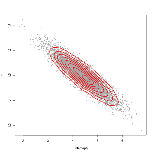
The large spread in the points (from top left to bottom right) is illustrative of greater uncertainty in the intercept term than in \( \hat{\beta}_x \).
As I said earlier, each point on the plot represents a valid model consistent with the estimates we achieved for the sample of data used to fit the model. If we were to multiple the second column of sim with the observed data and add on the first column of sim, we’d obtain fitted values for the observed x values for 5000 simulations from the fitted model as shown in the plot below
> plot(y ~ x, data = dat)
> set.seed(42)
> take <- sample(nrow(sim), 50) ## take 50 simulations at random
> fits <- cbind(1, dat$x) %*% t(sim[take, ])
> matlines(dat$x, fits, col = "#A9A9A97D", lty = "solid", lwd = 2)
> abline(mod, col = "red", lwd = 1)
> matlines(dat$x, predict(mod, interval = "confidence")[,-1], col = "red", lty = "dashed")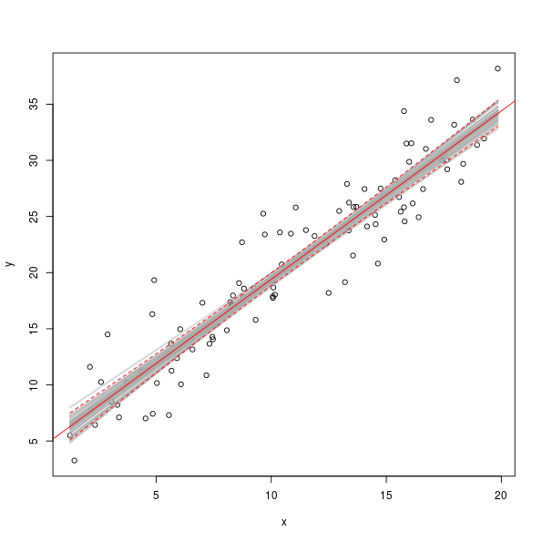
The grey lines show the model fits for a random sample of 50 pairs of coefficients from the set of simulated values.
Posterior simulation for additive models
You’ll be pleased to know that there is very little difference (non really) between what I just went through above for a simple linear regression and what is required to simulate from the posterior distribution of a GAM. However, instead of dealing with two or just a few regression coefficients, we now have to concern ourselves with the potentially larger number of coefficients corresponding to the basis functions that combine to form the fitted splines. The only practical difference is that instead of multiplying each simulation by the observed data4 with mgcv we generate the linear predictor matrix for the observations and multiply that by the model coefficients to get simulations. If you’ve read the previous post you should be somewhat familiar with the lpmatrix now.
Before we get to posterior simulations for the derivatives of the CET additive model fitted earlier, let’s look at some simulations for the trend term in that model, m2. If you look back at an earlier code block, I created a grid of 200 points over the range of the data which we’ll use to evaluate properties of the fitted model. This is in object pdat. First we generate the linear predictor matrix using predict() and grab the model coefficients and the variance covariance matrix of the coefficients
> lp <- predict(m2$gam, newdata = pdat, type = "lpmatrix")
> coefs <- coef(m2$gam)
> vc <- vcov(m2$gam)
Next, generate a small sample from the posterior of the model, just for the purposes of illustration; we’ll generate far larger samples later when we estimate a confidence interval on the derivatives of the trend spline.
> set.seed(35)
> sim <- mvrnorm(25, mu = coefs, Sigma = vc)
The linear predictor matrix, lp, has a column for every basis function, plus the constant term, in the model, but because the model is additive we can ignore the columns relating to the nMonth spline and the constant term and just work with the coefficients and columns of lp that pertain to the trend spline. Let’s identify those
> want <- grep("Time", colnames(lp))Again, a simple bit of matrix multiplication gets us fitted values for the trend spline only
> fits <- lp[, want] %*% t(sim[, want])
> dim(fits) ## 25 columns, 1 per simulation, 200 rows, 1 per evaln point
[1] 200 25We can now draw out each of these posterior simulations as follows
> ylims <- range(fits)
> plot(Temperature ~ Date, data = cet, pch = 19, ylim = ylims, type = "n")
> matlines(pdat$Date, fits, col = "black", lty = "solid")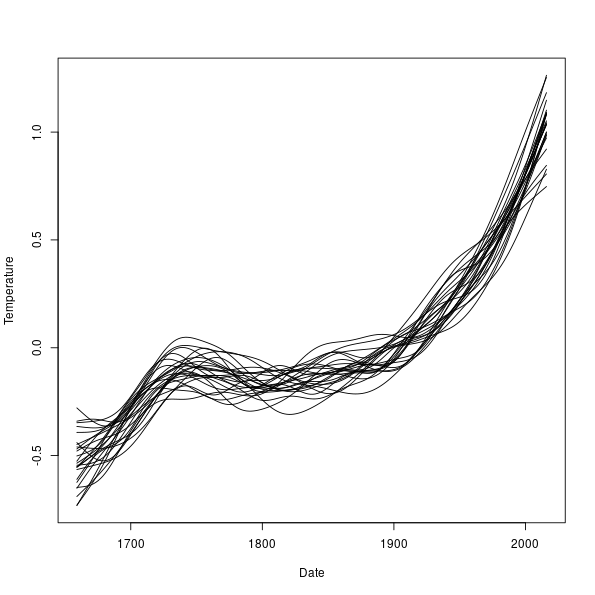
Posterior simulation for the first derivatives of a spline
As we saw in the previous post, the linear predictor matrix can be used to generate finite differences-based estimates of the derivatives of a spline in a GAM fitted by mgcv. And as we just went through, we can combine posterior simulations with the linear predictor matrix. The main steps in the process of computing the finite differences and doing the posterior simulation are
X0 <- predict(mod, newDF, type = "lpmatrix")
newDF <- newDF + eps
X1 <- predict(mod, newDF, type = "lpmatrix")
Xp <- (X1 - X0) / eps
where two linear predictor matrices are created, offset from one another by a small amount eps, and differenced to get the slope of the spline, and
for(i in seq_len(nt)) {
  Xi <- Xp * 0
  want <- grep(t.labs[i], colnames(X1))
  Xi[, want] <- Xp[, want]
  df <- Xi %*% t(simu[, want])    # derivatives
}
which loops over the terms in the model, selects the relevant columns from the differenced predictor matrix, and computes the derivatives by a matrix multiplication with the set of posterior simulations. simu is the matrix of random draws from the posterior, multivariate normal distribution of the fitted model’s parameters. Note that the code in derivSimulCI() is slightly different to this, but it does the same thing.
To cut to the chase then, here is the code required to generate posterior simulations for the first derivatives of the spline terms in an additive model
> fd <- derivSimulCI(m2, samples = 10000)fd is a list, the first n terms of which relate the the n terms in the model. Here n = 2. The names of the first two components are the names of the terms referenced in the model formula used to fit the model
> str(fd, max = 1)List of 5
$ nMonth :List of 2
$ Time :List of 2
$ gamModel:List of 31
..- attr(*, "class")= chr "gam"
$ eps : num 1e-07
$ eval : num [1:200, 1:2] 1 1.06 1.11 1.17 1.22 ...
..- attr(*, "dimnames")=List of 2
- attr(*, "class")= chr "derivSimulCI"As I haven’t yet written a confint() method, we’ll need to compute the confidence interval by hand, which is no bad thing of course! We do this by by taking two extreme quantiles of the distribution of the 10,000 posterior simulations we generated for the first derivative at each of the 200 points we wanted to evaluate the derivative. One of the reasons I did 10,000 simulations is that for a 95% confidence interval we only need sort the simulated derivatives in ascending order and extract the 250th and the 9750th of these ordered values. In practice we’ll let the quantile() function do the hard work
> CI <- lapply(fd[1:2],
+              function(x) apply(x$simulations, 1, quantile,
+                                probs = c(0.025, 0.975)))
CI is now a list with two components, each of which contains a matrix with two rows (the two probability quantiles we asked for) and 200 columns (the number of locations at which the first derivative was evaluated).
There is a plot() method, which by default produces plots of all the terms in the model and includes the simultaneous point-wise confidence interval as well
> plot(fd, sizer = TRUE)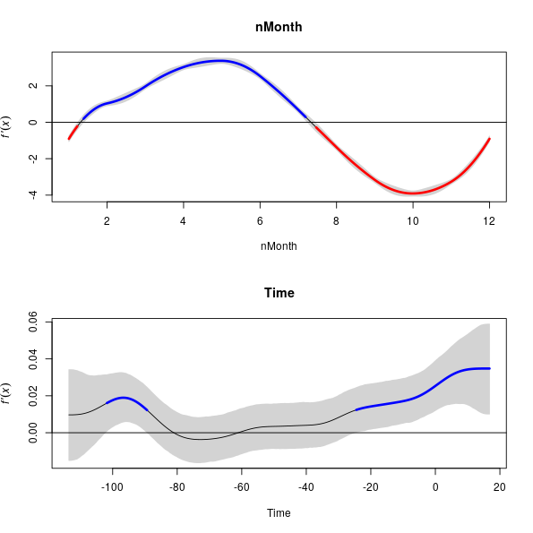
Wrapping up
derivSimulCI() computes the actual derivative as well as the derivatives for each simulation. Rather than rely upon the plot() method we could draw our own plot with the confidence interval. To extract the derivative of the fitted spline use
> fit.fd <- fd[[2]]$derivand then produce a plot with the actual derivative, the 95% simultaneous point-wise confidence interval, and 20 of the derivatives for the posterior simulations, we can use
> set.seed(76)
> take <- sample(nrow(fd[[2]]$simulations), 20)
> plot(pdat$Date, fit.fd, type = "l", ylim = range(CI[[2]]), lwd = 2)
> matlines(pdat$Date, t(CI[[2]]), lty = "dashed", col = "red")
> matlines(pdat$Date, fd[[2]]$simulations[, take], lty = "solid",
+          col = "grey")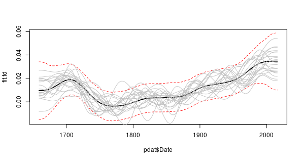
It is a little bit more complex than this, of course. If you allow
gam()to select the degree of smoothness then you need to fit a penalized regression. Plus, the time series models fitted to the CET data aren’t fitted viagam()but viagamm(), where we are using the observation that a penalized regression can be expressed as a linear mixed model, with random effects being used to represent some of the penalty terms. If you specify the degree of smoothing to use, these complications go away.↩The (squares of the) standard errors are on the diagonal of the VCOV, with the relationship between pairs of parameters being contained in the off-diagonal elements.↩
in practice. I suspect it is not quite so simple if one had to sit down and implement it…↩
or a set of new values at which you want to evaluate the confidence interval↩


